data_prepared
观察数据,进行数据分析
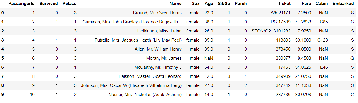
1 | train = pd.read_csv(r'train.csv') |
PassengerId (ID)
共891个不同值,因此无价值,可以考虑删除
Survived (是否生存)
很明显的label标签,也是我们需要预测的对象
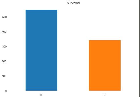
1 | train['Survived'].value_counts().plot.bar(title = 'Survived') |
Pclass(船舱等级)
生成一张关于Pclass的生存人数图看看
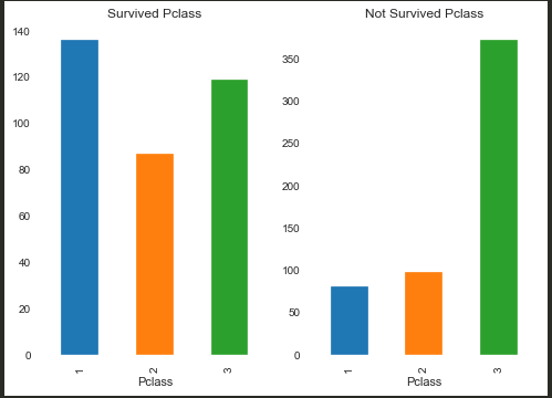
1 | Survived_Pclass = train[train.Survived==1].groupby(train.Pclass).Survived.count() |
发现Pclassd对于存活率还是有比较大的影响的,因此我们可以通过计算该特征的IV判断是否选择
经过计算,该特征的IV为:0.5006200325081741,因此使用该特征
Name(姓名)
通过数据集发现,Name看上去非常的杂乱无章,因为每个人的名字都可能不同,但是仔细研究,依旧可以尝试提取Name中的特征。
例如第一个Name:Braund, Mr. Owen Harris ,可以尝试提取其中的 Mr. 作为特征
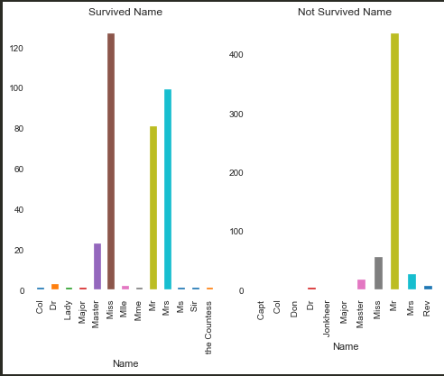
1 | train['Name'] = train['Name'].str.split('.').str.get(0) |
粗略一看其实也是有关联的,例如Miss存活率就比较高,接下来计算IV值
仔细观察可以发现有些值不是两者都有的,对于这些值我们是无法计算WOE的,因此首先去除掉这些值:
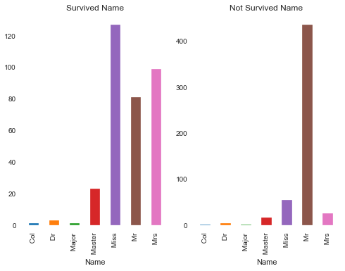
1 | train_name = train.copy() |
然后通过这个再去计算IV值:1.526927503266331
Sex(性别)
生成一张关于性别的生存人数图看看:
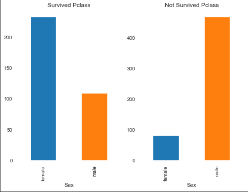
1 | Survived_Sex = train[train.Survived==1].groupby(train.Sex).Survived.count() |
很明显看到女性的存活率比男性高,再来算算IV值:1.3371613282771198
Age(年龄)
因为Age是一个连续的变量,因此如果直接采用柱状图会导致无法分析,因此先对Age进行分组,令每10年为一段,共分成10段,对这10段进行分析:
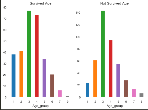
1 | train.dropna(inplace = True,subset = ['Age']) |
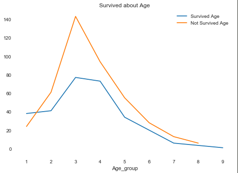
发现Age对Survived影响还是挺大的,再来看看IV值:0.3074963748595815,可以选择此特征值
SibSp(旁系)
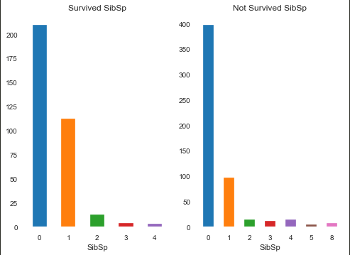
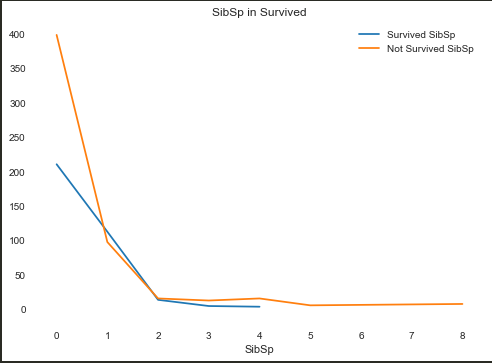
1 | Survived_SibSp = train[train.Survived==1].groupby(train.SibSp).Survived.count() |
IV:0.14091013517926007
Parch(直系亲友)
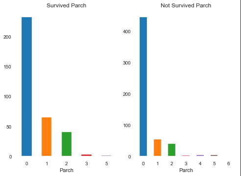
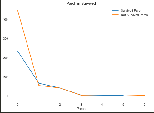
IV:0.1147797445933584
Ticket(票编号)
原以为看数据觉得Ticket应该是一个无用的数据,但是作图一分析,居然可以当作有用信息:
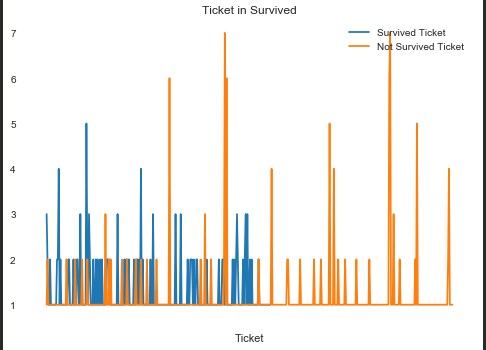
虽然大部分的编号是不一样的,但是依旧有一部分的编号是相同的,选择其中既有正例又有反例的部分做IV,课可以得到IV值:0.2421326661022386
不过经过这么剔除后,原数据大小891就变成了127条,损失太多,是否使用有待考虑。
Fare(票价)
在这个数据集中,票价最高512.3292,最低0,共有248种不同的票价,将这些票价分成25组再作图:
(分成25份分法:最高最低值均分25份)

1 | train['Fare_group'] = train['Fare']/((train['Fare'].max()+0.001)/25) + 1 |
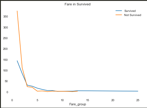
发现票价越低存活率越低,大胆猜测票价可能受到船舱等级的影响
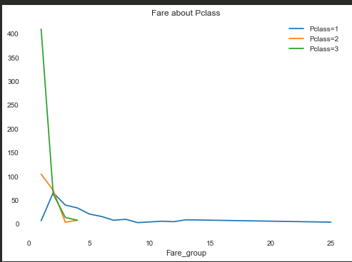
查图,果然票价越低,乘坐Pclass=3的船舱的概率越大
Cabin(客舱编号)
这个属性的数据缺失严重,所有891条数据中,只有204条数据是有效的,其余数据均缺失,暂时不采用该数据
Embarked(上船的港口编号)
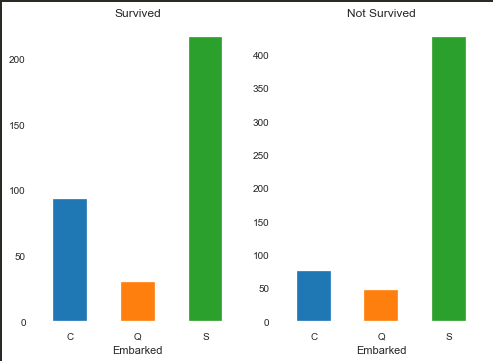
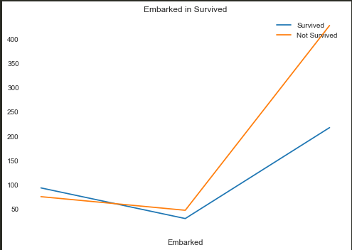
IV:0.12278149648986617
这个属性相对于别的属性利用价值偏小
缺失值处理
在处理整个数据的时候,发现有些数据有残缺,需要进行缺失值处理:
V1
对于Age参数,采用平均值填充,
对于Cabin,取消该列,
对于Embarked,暂时发现价值偏小,因此暂时取消该值
V2
在处理缺失值之前,先总结一下V1版本:
· 首先是Age的处理,直接采用平均值太过暴力
· 其次是Cabin的处理和Embarked的处理,直接取消会不会产生影响
· 对于Name属性的编码出现了错误,直接使用 lab.fit_transform 会产生编码错误
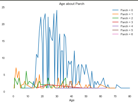
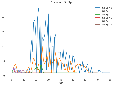
· 对于SibSp 属性和 Parch 属性,感觉在一定程度上有重复
优化1(Age)
相对于V1来说,Age直接采用平均值填充未免太过暴力,因此考虑别的填充方式。
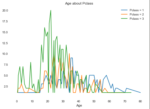
首先我们需要查看Age和别的属性之间的关系:
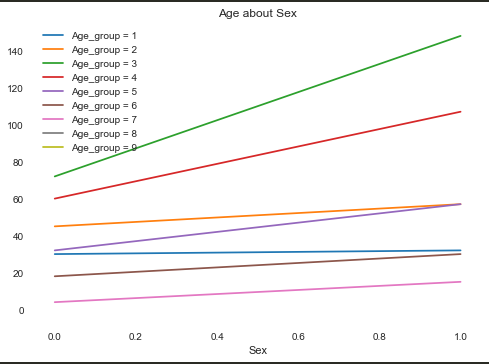
(Sex只有0和1两个属性)根据上图可以发现,在每个年龄段,Sex为1的人数都大于Sex为0的人数
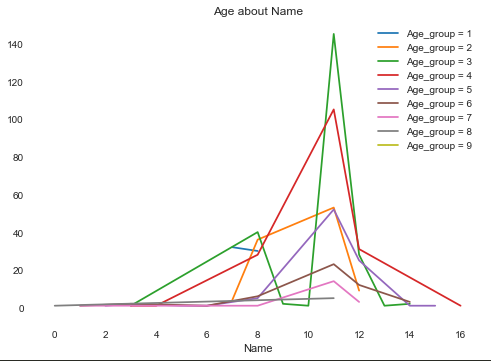
虽然这张图看上去很杂乱,但是还是可以发现一些规律
因为Fare是连续值,因此将Fare分成25份之后再查看Age的分布情况:
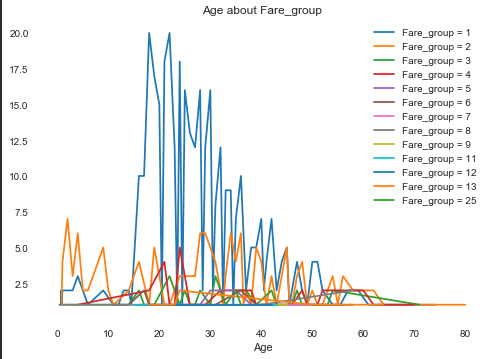
因此考虑使用预测的方式来对Age进行填充。
在这个版本中采用对Age分组,然后采用分类的方式(或许以后可以考虑回归的版本)。
优化2(Cabin)
对于Cabin属性,缺失值确实太多了,如果把Cabin属性中的缺失部分记为X,非缺失部分取其首位字母,作图看看:
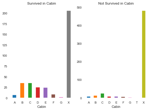
预估IV:0.4675285868289105 因此可以尝试将缺失值如此处理
优化3(Embarked)
对于Embarked,也尝试使用,因缺失值较少,采取随机赋值的方式
优化4(Name编码)
提取出Name中的所有不同值,依次进行编码,如果test中出现了train以外的,统一归为一类
(还有个问题:在name中有些name的个数为1,这样的样本是否可以结合起来)
针对上面这个问题,采取:将train中出现个数为个位数的归为一类,和test出现了train以外的归在一起
优化5(SibSp 和 Parch)
在这方面采用多加一个Family_size属性,其值为SibSp和Parch之和
优化6(Name属性提取)
在Name属性中提取了Mr.的内容,但是Name属性中还有姓氏,提取出姓氏形成新的属性Surname
在新属性Surname中,采用二分类,具有相同姓氏的归为1,否则为0
优化7(模型优化)
同时在模型的实现方面,一方面采用随机森林对所有属性进行训练,同时训练多个随机森林,对多种属性组和进行训练,最后按照不同的权重比例取值
V3
· 有了Family_size之后感觉SibSp和Parch有点多余,因此选择删除
· Cabin选择缺失值插入X,Cabin损失值太多,最终还是选择放弃该属性
· 修改了一下随机森林训练的属性
实现
V1
采用随机森林,缺失值处理采用V1的处理方式,采用的特征组合为:Pclass,Name,Sex,Age,SibSp,Parch,Fare
1 | import pandas as pd#导入数据文件 |
该实验在kaggle上面评分0.71291
V2
对于Age的预测采用的属性:Pclass,Name,Sex, SibSP, Parch, Fare_group, Family_size,Embarked,Surname,Cabin
采用多个随机森林按照不同的权重取值,按照不同的属性组合进行随机森林的训练
随机森林训练:
1 | ['Pclass','Fare'], |
共计生成了27个预测结果,采用少数服从多数,阈值大约为18 ~ 19。对于每一个真实的结果,当含有1的个数大于等于阈值时,认为其是可靠的预测结果。
1 | import pandas as pd#导入数据文件 |
上述代码部分省略了数据的预处理部分
上述模型在kaggle上为0.799
kaggle上面震荡大约在0.770~0.799(可能再偏低点或偏高点)
V3
随机森林训练:
1 | ['Pclass','Fare'], |
1 | import pandas as pd#导入数据文件 |
kaggle: 0.80382
此版本基于V2版本的数据,在kaggle上提交大约会在0.794~0.803左右震荡(可能还会再偏高点或偏低点)
other
about IV and WOE:
1 | def calcWOE(dataset,col,targe): |
refer: https://blog.csdn.net/weixin_38940048/article/details/82316900